
Non-invasive continuous health monitoring can greatly improve the efficiency of our healthcare systems, and help save many lives. As we’ve seen in a previous post, Atrial Fibrillation (or AFib), an abnormal heart rhythm, increases the risk of stroke and heart failure. With the proper prevention and diagnosis, we can put a stop to many of the deaths that result from cardiovascular diseases — the number 1 cause of death worldwide.
One promise is the use of everyday wearables to track heart rhythm. It gives cardiologists the chance to monitor problems at a distance, in a way that is non-invasive and easy for the patient.
Automation plays a big role. Smart software and algorithms are responsible for alerting physicians if something is wrong. In this post we’ll develop one such algorithm: a neural network that can detect AFib from a few seconds recording of a single lead ECG, like the one you can find on an Apple Watch.
We’ll roughly follow the paper Convolutional Recurrent Neural Networks for Electrocardiogram Classification. We’ll use Pytorch and the PhysioNet dataset.
The PhysioNet dataset
The publicly available PhysioNet/CinC Challenge 2017 data set contains 8,528 single lead ECG recordings of length ranging from 9 to 61 seconds, sampled at 300Hz.
Each recording is labeled with one of the classes “normal rhythm”, “AF rhythm”, “other rhythm”, and “noisy recording”. From now on we’ll refer to these classes as “N”, “A”, “O”, and “~” respectively.
If you’d like to follow along, go ahead and download the training data. The data are provided as EFDB-compliant Matlab V4 files (each including a .mat file with the ECG data and a .hea file with the waveform information). The REFERENCE.csv has the labels.
For a detailed description of the dataset, see this paper.
Let’s plot 10 seconds of a sample recording for each class:
<script src="https://gist.github.com/pbnsilva/b5742f440ea013ed8a210a48fa0785b3.js"></script>
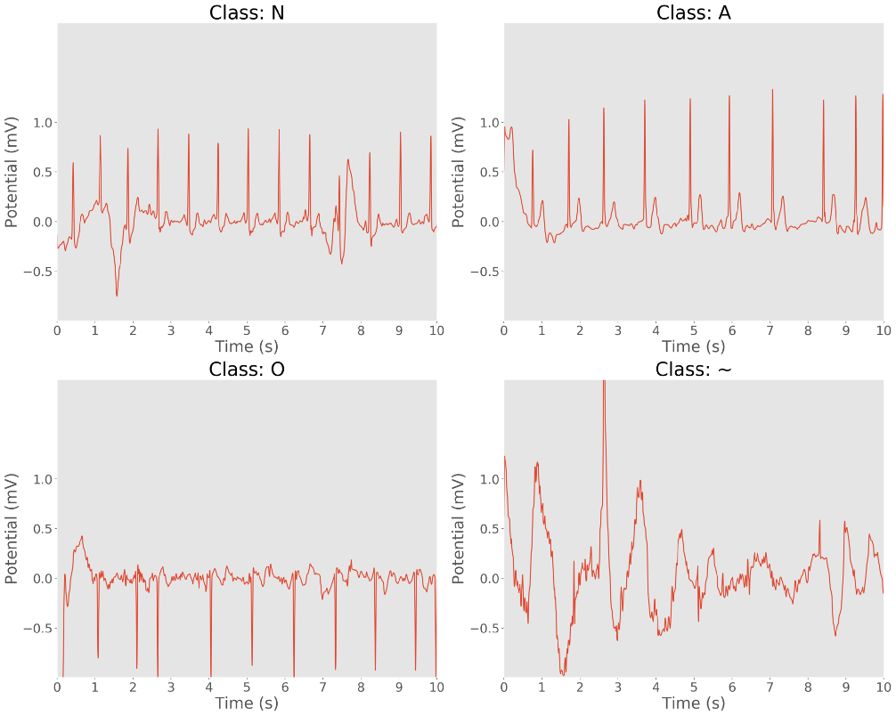
10 second samples of ECG recordings. Clockwise: normal rhythm, AF rhythm, noisy recording, and other rhythm.
Preparing the data
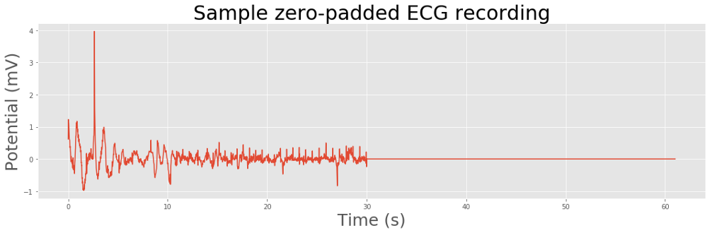
Our neural network expects all the input data to be of the same size. Since our recordings have variable lengths, we’ll pad the ECGs with zeros to create sequences of consistent lengths.
def zero_pad(data, length):
    extended = np.zeros(length)
    siglength = np.min([length, data.shape[0]])
    extended[:siglength] = data[:siglength]
    return extended

# plot a sample
data = sio.loadmat('training2017/A00001.mat')['val'][0]

# 61 seconds is the maximum length in our dataset
data = zero_pad(data, max_length*freq)

plt.figure(figsize=(15, 5))
plt.title('Sample zero-padded ECG recording', fontsize=30)
plt.xlabel('Time (s)', fontsize=25)
plt.ylabel('Potential (mV)', fontsize=25)
plt.plot(np.arange(0, data.shape[0])/300, data/1000)
<a href="https://gist.github.com/pbnsilva/516f5c4eb0ff9ee995cdf12c2df039c0/raw/a30ece3f92534b890fcc6718b847fd141acf275c/1d_ecg2_zeropad.py">view raw</a><a href="https://gist.github.com/pbnsilva/516f5c4eb0ff9ee995cdf12c2df039c0#file-1d_ecg2_zeropad-py">1d_ecg2_zeropad.py</a> hosted with ❤ by <a href="https://github.com/">GitHub</a>
Electrocardiograms are representations of the periodic cardiac cycle. To make sense of an ECG we need to look at the frequency information, and how it changes over time.
STFT and the spectrogram
We can apply the discrete Fourier transform (DFT) to extract the frequency information and obtain the power spectrum, but this will obfuscate the time information. Instead, we can apply a form of the Fourier transform called short-time Fourier transform (STFT). Rather than taking the DFT of the whole signal in one go, we split the signal into small pieces and take the DFT of each individually, in a sliding-window fashion. Then, we plot it as a spectrogram, which is a clever way to visualize the frequency, power, and time in a single image. It is basically a two-dimensional graph, with a third dimension represented by colors. The amplitude of a particular frequency at a particular time is represented by the color, with dark blues corresponding to low amplitudes and brighter colors up through red corresponding to progressively stronger amplitudes.
To optimize the dynamic range of the frequency, it is also useful to apply a logarithmic transform. In fact, other reports showed that the logarithmic transform considerably increases the classification accuracy.
from scipy import signal

def spectrogram(data, fs=300, nperseg=64, noverlap=32):
    f, t, Sxx = signal.spectrogram(data, fs=fs, nperseg=nperseg, noverlap=noverlap)
    Sxx = np.transpose(Sxx, [0, 2, 1])
    Sxx = np.abs(Sxx)
    mask = Sxx > 0
    Sxx[mask] = np.log(Sxx[mask])
    return f, t, Sxx

f, t, Sxx = spectrogram(np.expand_dims(data, axis=0))

plt.figure(figsize=(15, 5))
xticks_array = np.arange(0, Sxx[0].shape[0], 100)
xticks_labels = [round(t[label]) for label in xticks_array]
plt.xticks(xticks_array, labels=xticks_labels)
plt.xlabel('Time (s)', fontsize=25)
plt.ylabel('Frequency (Hz)', fontsize=25)
plt.imshow(np.transpose(Sxx[0]), aspect='auto', cmap='jet')
plt.gca().invert_yaxis()
<a href="https://gist.github.com/pbnsilva/724f090423ef77b17e9e03917ddc93c7/raw/f113e99ebe172aa5dc3bcbe24436bb24cd6d4626/1d_ecg3_spectrogram.py">view raw</a><a href="https://gist.github.com/pbnsilva/724f090423ef77b17e9e03917ddc93c7#file-1d_ecg3_spectrogram-py">1d_ecg3_spectrogram.py</a> hosted with ❤ by <a href="https://github.com/">GitHub</a>
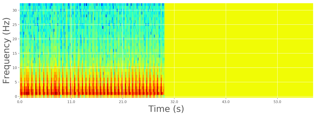
Log-spectrogram of zero-padded sample ECG recording
Custom dataset
Pytorch has some neat data utilities to make it easy to feed data into our model. We’ll define a custom data set that will be responsible for reading our raw ECG data and transform it in the ways we discussed before.
<script src="https://gist.github.com/pbnsilva/cb86c9f043a7c7e780449cc7dc25f17a.js"></script>
Now we can use this dataset to create two data loaders, one for our training job and another for validation:
<script src="https://gist.github.com/pbnsilva/2aa5fff6b30127136d7d6ab4e338bbaa.js"></script>
Creating the model
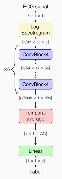
The model we’ll implement (see paper here) will take our spectrograms as input, and pass them through a stack of convolutional layers for feature extraction. Then, because the convolutional blocks produce variable length outputs, we aggregate the features across time by simply averaging them. Finally, we apply a linear classifier to compute the class probabilities, and assign one of the 4 labels.
We’re going to need several convolutional blocks, so we can define a module to make it easy to reuse:
<script src="https://gist.github.com/pbnsilva/c5692364299a2676713537a7485b9f50.js"></script>
Finally, we can define the full network:
<script src="https://gist.github.com/pbnsilva/77872b9f06bcd347afe75d0e2884d6b9.js"></script>
Training
Now we’re ready to train our model:
<script src="https://gist.github.com/pbnsilva/f378e363e482da57365abc72ce3f3273.js"></script>
Plotting the training and validation loss and accuracy:
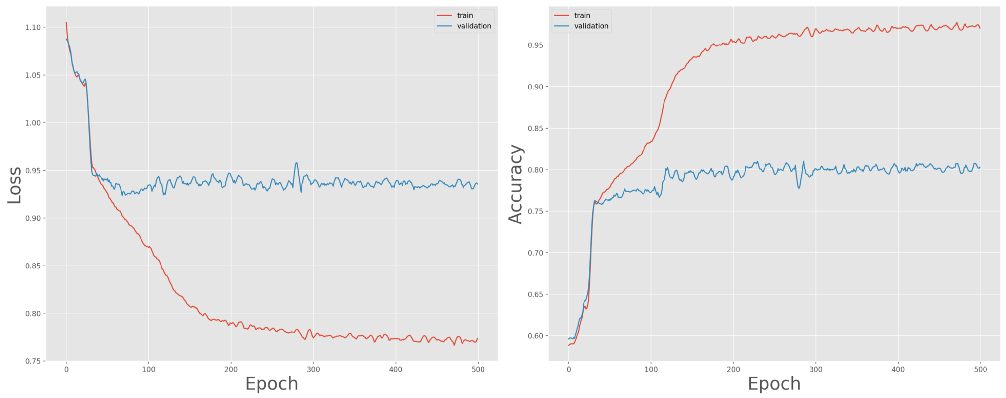
Training and validation loss (left) and accuracy (right) over 500 epochs
We can expect the model to overfit due to the large number of parameters in the network architecture. Also, notice how the performance on the training set quickly diverges from that of the validation set. The paper we’re following proposes two data augmentation techniques to deal with this: dropout bursts and random resampling.
The dropout bursts emulate periods of weak signal, for example due to bad contact of the ECG lead. It works by selecting time instants uniformly at random and setting the ECG signal values in a 50ms vicinity of those time instants to 0.
Random resampling emulates a broader range of heart rates by uniformly resampling the ECG signals such that the heart rate of the resampled signal is uniformly distributed on the interval [60, 120] bpm. These emulated heart rates may be unrealistically high or low due to the assumption of an 80bpm heart rate independently of the signal.
Applying these data augmentation techniques and retraining yields much better results:
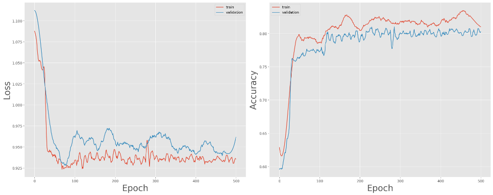
Training and validation loss (left) and accuracy (right) over 500 epochs, with data augmentation
The model converges fairly well, closing in on 80% accuracy for the validation set.
Conclusion
We’ve shown that we can accurately detect Atrial Fibrillation from a single lead ECG. This is one of the many sensors we have available today on our everyday wearables, and just one of many ways it can be used. For example, we can use a heart rate monitor to diagnose sleep apnea, or show infection. The fact that you’re wearing it all the time, means you’ll make findings that would be missed in traditional health screenings. With constant monitoring, doctors can discover clinically actionable information earlier and at a broader scale. This means acting on problems in time, preventing diseases before they become truly problematic, and saving trips to the hospital.
Other sensors
ECG gives us precision, but the measurements need to be taken actively. For example, on the Apple Watch, you must rest your arm and place your finger on the sensor. It would be great if heart rhythm could be monitored passively. This is where Photoplethysmography (PPG) comes in. A PPG uses light sensors to measure the changes in volume of the capillaries under the skin. A LED shines light against the skin; some of it is reflected and scattered back onto the photodiode; the amount that is reflected changes as the heart beats, which determines the heart rate. Devices that record PPG have limitations, but the technique shows promise for the detection of Atrial Fibrillation (see here and here).
Merge this with other sensors, like GPS, gyroscopes, and accelerometers, and you have a powerful diagnosis system on your wrist. It can detect problems as they’re happening, and let your doctor know in time.
Consider also the “smart toilet”, that could someday detect a range of disease markers in stool and urine, including colorectal and urologic cancer. Furthermore, it could help understand and monitor the spread of viral disease on a wider scale, including diseases like Covid-19.
A paradigm shift
We’re just at the beginning of a paradigm shift that is hitting healthcare : continuous health monitoring.
Being proactive rather than reactive could prove a more cost-effective approach to healthcare — especially at a time when many health services are struggling with budget cuts and a growing, and aging, population.
Ultimately, we want to shift the practice of medicine from treating people when they are ill to a focus on keeping them healthy by predicting disease risk and catching disease before it is symptomatic.
Connect
At 1D.works we’re excited about the potential of AI to improve people’s lives. Healthcare is just one of the largely unexplored territories we’re invested in. If you think you can benefit from a decade-long experience of applying machine learning to business processes.
Explore our AI-First Product Development service. Read how we built an AI-Powered Fetal Monitoring Solution.